In our initial post, we introduced the InterBase Model Context Protocol (MCP) Server – a tool engineered with Delphi to bridge Large Language Models (LLMs) with InterBase databases. In this follow-up, we are opening our playground notebook: a real, step-by-step session where I used ChatGPT to interact directly with an InterBase database instance using InterBase MCP tools and agentic skills.

See below what we tried so far and the achieved results:

1. Discovering the schema

Prompt: List all tables in the database, then show each table’s columns, data types, nullability, primary keys, foreign keys, and indexes.

The database contains ten user tables:

Table	Primary key	Purpose
COUNTRY	COUNTRY	Country and currency reference data
CUSTOMER	CUST_NO	Customer contact and location data
DEPARTMENT	DEPT_NO	Organizational hierarchy and budgets
EMPLOYEE	EMP_NO	Employees, jobs, departments, and salaries
EMPLOYEE_PROJECT	EMP_NO, PROJ_ID	Employee-to-project bridge
JOB	JOB_CODE, JOB_GRADE, JOB_COUNTRY	Job definitions and salary ranges
PROJECT	PROJ_ID	Projects, products, and team leaders
PROJ_DEPT_BUDGET	FISCAL_YEAR, PROJ_ID, DEPT_NO	Project budgets by department and year
SALARY_HISTORY	EMP_NO, CHANGE_DATE, UPDATER_ID	Employee salary changes
SALES	PO_NUMBER	Orders, sales representatives, quantities, and values

The catalog inspection identified 13 foreign-key relationships. The central transactional table is SALES, which references CUSTOMER through CUST_NO and EMPLOYEE through SALES_REP. The employee, department, job, and project tables form the core organizational model. The complete column-level output was saved as schema-document.md. It includes data types, nullability, defaults, constraints, indexes, and a relationship summary.

2. Generating the schema document and ER diagram

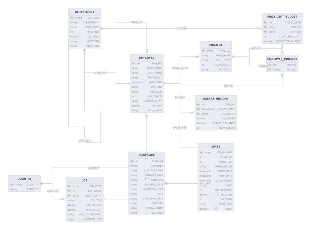
Prompt: Generate a Markdown schema document, then create a hierarchical ER diagram showing every column, data type, nullability rule, primary key, and foreign-key relationship.

The initial attempts to generate an ER diagram didn’t go well, to put it plainly — the diagrams didn’t match the format or level of detail an architect would expect. After some research, I fed the AI agent specific modeling skills from this project: https://github.com/imxv/Pretty-mermaid-skills

With that, we achieved very promising results, and I believe there’s room to push further. See below:

• schema-er.mmd, the Mermaid source.
• schema-er.svg, the rendered vector diagram.

3. Inspecting customer data

Prompt: Show the data stored in the CUSTOMER table.

The table contained 15 customers. The following compact view shows the identifying and location fields retrieved during the experiment:

Customer no.	Customer	City	Region	Country	On hold
1001	Signature Design	San Diego	CA	USA
1002	Dallas Technologies	Dallas	TX	USA	*
1003	Buttle, Griffith and Co.	Boston	MA	USA
1004	Central Bank	Manchester		England
1005	DT Systems, LTD.	Central Hong Kong		Hong Kong
1006	DataServe International	Ottawa	ON	Canada
1007	Mrs. Beauvais	Pebble Beach	CA	USA
1008	Anini Vacation Rentals	Lihue	HI	USA
1009	Max	Turtle Island		Fiji	*
1010	MPM Corporation	Tokyo		Japan
1011	Dynamic Intelligence Corp	Zurich		Switzerland
1012	3D-Pad Corp.	Paris		France
1013	Lorenzi Export, Ltd.	Milan		Italy
1014	Dyno Consulting	Brussels		Belgium
1015	GeoTech Inc.	Den Haag		Netherlands

Two customers, Dallas Technologies and Max, were marked as on hold.

4. Finding the top customers by sales value

Prompt: Write and run an InterBase query that returns the ten customers with the highest total sales value.

The working InterBase query was:

SELECT C.Cust_no,
       C.Customer,
       Sum(S.Total_value) AS Total_sales_value
FROM Customer C
JOIN Sales S ON S.Cust_no = C.Cust_no
GROUP BY C.Cust_no,
         C.Customer
ORDER BY Total_sales_value DESC ROWS 1 TO 10

Result

Rank	Customer no.	Customer	Total sales value
1	1001	Signature Design	1,045,610.12
2	1012	3D-Pad Corp.	463,000.47
3	1006	DataServe International	400,008.00
4	1011	Dynamic Intelligence Corp	121,980.72
5	1004	Central Bank	75,000.00
6	1003	Buttle, Griffith and Co.	39,582.12
7	1002	Dallas Technologies	35,450.50
8	1008	Anini Vacation Rentals	25,000.00
9	1010	MPM Corporation	21,195.40
10	1005	DT Systems, LTD.	14,980.00

Signature Design was the clear leader, accounting for more than twice the sales value of the second-ranked customer.

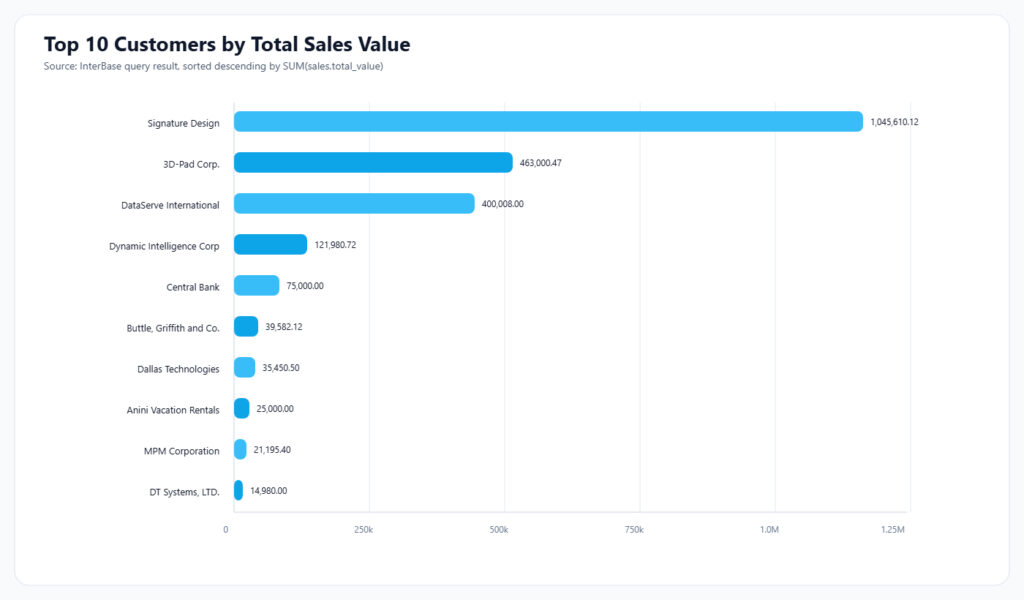
Prompt: Present the same result as a chart.

The chart was saved as top-customers-chart.svg.

5. Building a database dashboard

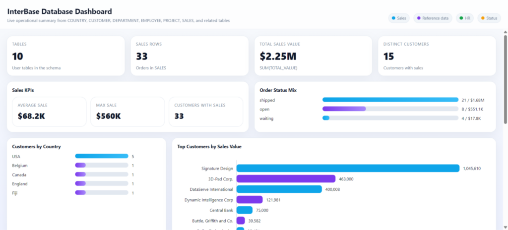
Prompt: Create a dashboard that summarizes the database’s most relevant operational and analytical data.

The resulting database-dashboard.html combined schema counts, sales KPIs, order status, customer geography, top customers, employee salary statistics, department headcount, and table row counts.

6. Constructing a multi-table stress query

Prompt: Create a complex query that joins as many related tables as practical so we can inspect database performance.

The final test query joined nine of the ten tables. It used SALES as the driving table and followed relationships into customer, employee, department, job, project, project budget, salary history, and country data:

SELECT S.Order_status,
       Co.Country AS Country_name,
       Co.Currency,
       D.Department,
       J.Job_title,
       P.Product,
       Count(*) AS ROW_COUNT,
       Count(DISTINCT S.Po_number) AS Order_count,
       Count(DISTINCT C.Cust_no) AS Customer_count,
       Count(DISTINCT E.Emp_no) AS Sales_rep_count,
       Count(DISTINCT P.Proj_id) AS Project_count,
       Sum(S.Qty_ordered) AS Total_qty_ordered,
       Sum(S.Total_value) AS Total_sales_value,
       Avg(S.Total_value) AS Avg_sales_value,
       Min(S.Total_value) AS Min_sales_value,
       Max(S.Total_value) AS Max_sales_value,
       Avg(E.Salary) AS Avg_sales_rep_salary,
       Avg(D.Budget) AS Avg_department_budget,
       Avg(B.Projected_budget) AS Avg_projected_budget,
       Avg(Sh.Percent_change) AS Avg_salary_change_pct,
       Max(Sh.Change_date) AS Last_salary_change
FROM Sales S
LEFT JOIN Customer C ON C.Cust_no = S.Cust_no
LEFT JOIN Employee E ON E.Emp_no = S.Sales_rep
LEFT JOIN Department D ON D.Dept_no = E.Dept_no
LEFT JOIN Job J ON J.Job_code = E.Job_code
AND J.Job_grade = E.Job_grade
AND J.Job_country = E.Job_country
LEFT JOIN Project P ON P.Team_leader = E.Emp_no
LEFT JOIN Proj_dept_budget B ON B.Proj_id = P.Proj_id
AND B.Dept_no = D.Dept_no
LEFT JOIN Salary_history Sh ON Sh.Emp_no = E.Emp_no
LEFT JOIN Country Co ON Co.Country = Coalesce(C.Country, E.Job_country)
GROUP BY S.Order_status,
         Co.Country,
         Co.Currency,
         D.Department,
         J.Job_title,
         P.Product
ORDER BY S.Order_status,
         Total_sales_value DESC,
         Customer_count DESC

7. Explaining the complex query plan

Prompt: Explain the execution plan for the multi-table query.

InterBase returned the following query plan:

PLAN SORT (SORT (JOIN (JOIN (JOIN (JOIN (JOIN (JOIN (JOIN (JOIN
(S NATURAL,C INDEX (RDB$PRIMARY22)),
E INDEX (RDB$PRIMARY7)),
D INDEX (RDB$PRIMARY5)),
J INDEX (RDB$PRIMARY2)),
P INDEX (RDB$FOREIGN13)),
B INDEX (RDB$FOREIGN18,RDB$FOREIGN19)),
SH INDEX (RDB$FOREIGN21)),
CO INDEX (RDB$PRIMARY1))))

The plan shows that:

• SALES was read with a natural scan (S NATURAL).
• Lookup tables used primary-key or foreign-key indexes.
• Two sort operations were required for grouping, distinct aggregates, and final ordering.

Because the query had no selective WHERE clause and aggregated the complete SALES table, a natural scan was reasonable.

8. Applying Metadata Changes/Optimizations

If permitted by your configuration, the tool is also capable of applying changes directly to the metadata. For this experiment, I first prompted the AI to present the execution plan for the following SQL statement:

Prompt: show the query plan for the following statement.

SELECT S.Po_number,
       S.Order_date,
       S.Order_status,
       S.Total_value
FROM Sales S
WHERE S.Order_date >= Cast('2023-01-01' AS DATE)
  AND S.Order_date < Cast('2024-01-01' AS DATE)
ORDER BY S.Order_date,
         S.Po_number;

InterBase returned the following query plan:

PLAN SORT ((S NATURAL))

InterBase performs a full SALES table scan (NATURAL) and then sorts the matching rows. No index is used.

Prompt: Now, suggest indexes that can be created in order to optimize the query execution.

The best index for this specific query is:

CREATE INDEX IDX_SALES_ORDER_DATE_PO ON SALES (ORDER_DATE, PO_NUMBER);

It supports:

• The range filter on ORDER_DATE.
• The ORDER BY ORDER_DATE, PO_NUMBER.
• Avoiding or reducing the full scan and explicit sort.

Prompt: Ok, go ahead and create the suggested index.

Created and verified:

CREATE INDEX IDX_SALES_ORDER_DATE_PO ON SALES (ORDER_DATE, PO_NUMBER);

Plan comparison:

Before: PLAN SORT ((S NATURAL)) 
After:  PLAN (S ORDER IDX_SALES_ORDER_DATE_PO)

InterBase now uses the index and no longer requires a natural scan or explicit sort.